The complexity class of #P problems

Recently, I had an assignment in one of my courses - Beyond NP-Completeness, to present the complexity class of #P (Sharp-P) problems based on L.G. Valiant’s paper on complexity of computing the permanent of a matrix.

This post is an attempt to explain the paper as I found very limited number of resources on the internet where this topic is discussed in detail, one of the sightings being a lecture by Professor Erik Demaine under MIT open courseware which can be found on youtube.

Before we begin, it is strongly recommended to familiarize yourself with the following:

• The classes P, NP, NP-Hard, NP-Complete
• Poly-time reductions
• The class FP
• The notion of an Oracle

So let’s begin with the permanent, which is defined for an n x n matrix A as:

Before proceeding, let’s understand what this means, and what we want to compute. \(\sigma\) is a permutation of the numbers {1, 2, 3, … n}. For example, for n = 5, if \(\sigma\) = {2, 5, 3, 4, 1}, then \(\sigma(1) = 2\), \(\sigma(2) = 5\), \(\sigma(3) = 3\) and so on. The summation, therefore, is over all \(\sigma\), which means we are doing the summation for all possible permutations, a total of them being \(n!\) (factorial of n). So it is evident, that when taking the product, which is inside the summation term, we must take one element from each row and each column of the matrix, and a total of n elements have to be picked, therefore exactly one element from each row and each column has to be picked.

A closer look at the permanent tells us that if we change all the negative signs in the expression of the determinant of a matrix to positive signs, it will indeed become the Permanent. To show this with an example: Consider the matrix,

The determinant of \(M\), \({\rm det}~M = (3 - 3) -2(2 - 1) + 4(6 - 3)\), while the permanent is: \((3 + 3) + 2(2 + 1) + 4(6 + 3)\), which is clearly obtainable by changing all negative signs in the determinant’s expression to positive. Surprisingly, though there exist efficient solutions to compute the determinant of a matrix, yet to compute the permanent, no algorithm that takes better than exponential time is known.

Valiant comments on the complexity of the problem of finding the permanent of a (0-1) matrix, for which he defines the class #P. To put it easily, #P problems are the counting problems associated with the decision problems in class NP. It is a class of function problems, and not decision problems (where the answer is a simple yes/no). An NP problem of the form “Does there exist a solution that satisfies X?” usually corresponds to the #P problem “How many solutions exist which satisfy X?”. Here goes the example of a #P problem: #SAT - Given a boolean formula \(\phi(x_1, x_2, ... x_n)\), find the number of assignments that satisfy \(\phi\). This is the counting version of the famous SAT problem which is known to be NP-complete.

Defining #P completeness

To define completeness in this class of problems, we need to bring in Oracle Turing Machines and the class FP. Oracle machines are those which have access to an oracle that can magically solve the decision problem for some language \(L \subseteq \{0, 1\}^*\). These machines with oracle access can then make queries of the form “Is \(q \in L\)?” in one computational step. We can generalize this to non-boolean functions by saying that a T.M. M has oracle access to a function \(f: \{0, 1\}^* \rightarrow \{0, 1\}^*\) if it is given access to the language \(L = \{(x, i) : f(x)_i = 1\}\). For every \(O \subseteq \{0, 1\}^*\), we denote \(P^O\) as the set of languages that can be decided by a polynomial-time DTM (Deterministic Turing Machine) with oracle access to O. As an example, consider the \(\overline{SAT}\) problem, which denotes the language of unsatisfiable boolean formulae. \(\overline{SAT}\) \(\in P^{SAT}\) because if we are given an oracle access to the SAT language, then we can solve an instance \(\phi\) of the \(\overline{SAT}\) problem in polynomial time, by asking “Is \(\phi \in SAT\)?” and negating the answer to that. Now we are ready to define #P completeness. A function \(f\) is said to be #P-complete if \(f \in \#P\) and \(\forall g \in \#P, g\) is in \(FP^f\) (Cook reduction).

Back to the problem

Now let’s get back to the permanent. We take a special case of the permanent problem where we put a constraint that the input matrix is a (0, 1) matrix, that is, all the entries of the given matrix are either 0 or 1. Let us look at this problem of finding the permanent of a binary matrix with a different perspective. Imagine that the given matrix A is an adjacency matrix of a bipartite graph \(G = (X, Y, E)\) where, \(X = \{x_1, x_2, ... x_n\}\) \(Y = \{y_1, y_2, ... y_n\}\) \(E = \{(x_i, y_j) : A_{ij} = 1\}\)

Now if we look at the term inside the summation, that is \(\prod{A_{i, \sigma(i)}}\) for \(i = \{1, 2, ... n\}\), we can try to imagine the value of this term as synonymous to a possible perfect matching in the bipartite graph represented by A. Why? Because we know that this term takes one element from each row and each column, so all vertices are covered in the term, and this term = 0, if any of the elements picked are 0. But in our adjacency matrix, 0 for row i and column j means that there is no edge between \(x_i\) and \(y_j\), so this term evaluates to 1 if and only if the selected elements form an edge cover (a perfect matching) for the given bipartite graph. So clearly, the whole term \({\rm Perm}\ A = \sum\prod A_{i, \sigma(i)}\) where the summation is over all \(\sigma\) represents the total number of perfect matchings in the bipartite graph represented by A. As finding the number of perfect matchings in a bipartite graph \(\in\) #P, therefore clearly, finding the permanent of a binary matrix \(\in\) #P.

Now we shall move on to prove the Valiant’s theorem which says that finding permanent for a binary matrix is #P-complete. We already proved it is in #P, so now all remains for us is to prove that it is in #P-Hard, that is all #P problems can be reduced to this problem in the way explained earlier in this post (where completeness is defined for #P problems). For this, we look at the problem of finding the permanent as a different graph problem.

Consider A = adjacency matrix of a weighted and directed graph with n nodes (We are talking about a general matrix now, not a binary matrix). We define two things now:

• Cycle Cover of a graph G: A set of cycles (subgraphs of G in which all vertices have indegree = 1 and outdegree = 1) which contains all vertices of G
• Weight of a cycle cover: Product of weights of edges involved in the cover

Now, with a good observation, we can conclude that \({\rm Perm}(A) = \sum W_{i}\) where \(W_i\) is the weight of the \(i^{th}\) cycle cover. We sum the weights of all possible cycle covers of the graph and it turns out to be equal to the permanent of the adjacency matrix. If this is hard to visualize, feel free to work out on an example having 3 or 4 nodes to let that sink in.

Proceeding with the proof, we will attempt to reduce an instance of the 3-SAT problem to an instance of the cycle cover problem. The methodology and examples are directly taken from the original paper. We begin with a boolean formula given to us in 3-CNF form. \(F = C_1 \wedge C_2 \wedge C_3 \wedge ... C_m\), a conjunction of m clauses where \(C_i = (y_{i1} \vee y_{i2} \vee y_{i3})\), a disjunction of 3 literals, where \(y_{ij} \in \{x_1, \overline{x_1}, x_2, \overline{x_2}, ... x_n, \overline{x_n}\}\), the set of variable and their negations.

We construct graph G by superposing the following the structures:

1. A Track \(T_k\) for each variable \(x_k\)
2. An Interchange \(R_i\) for each clause \(C_i\)
3. For each literal \(y_{ij}\) such that \(y_{ij} = x_k\) or \(\overline{x_k}\), a Junction \(J_{ik}\) at which interchange \(R_i\) and track \(T_k\) meet.
4. The interchanges also have internal junctions, which are exactly same as above

Example: Let’s take some formula F where: \(C_3 = (x_2 \vee \overline{x_5} \vee x_7)\) \(x_5\) occurs in \(C_2\) and \(C_5\) \(\overline{x_5}\) occurs in \(C_3\)

For this example, the following are the structures:

Track \(T_5\)	Interchange \(R_3\)

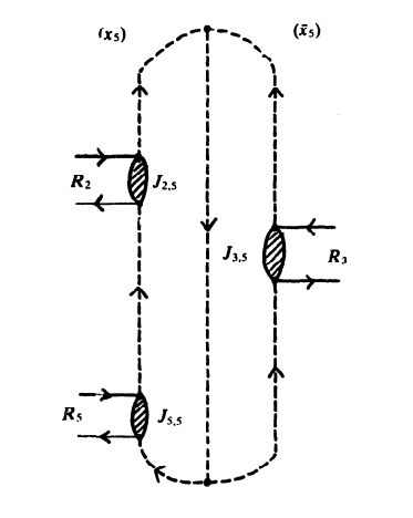The small shaded regions are the junctions, which are themselves a network of nodes and edges represented by the adjacency matrix,

Why this matrix is valued exactly with these numbers will be clear as we proceed. This is a very crucial part. Let’s note some important things:

• Each junction (represented by \(X\)) has external connections only via nodes 1 and 4
• Taking \(X(a; b)\) as the matrix leftover after deleting rows a and columns b, we note the following properties of the matrix \(X\):
  • \({\rm Perm}(X) = 0\).
  • \({\rm Perm}(X(1; 1)) = 0\).
  • \({\rm Perm}(X(4; 4)) = 0\).
  • \({\rm Perm}(X(1,4; 1,4)) = 0\).
  • \({\rm Perm}(X(1; 4)) = {\rm Perm}(X(4; 1)) = 4\).

Using these properties, we can draw very good insights. Let’s look at routes in the graph. A route is a cycle cover. If we consider all the routes which have the same set of edges outside of the junctions, then we can call a route bad if:

• It ignores a junction
  In this case, the cycle cover will have the ignored junction to be covered, so it will come separately as a product in the term. But \({\rm Perm}(X) = 0\), so it will make the whole term 0 and thus will not contribute to the cycle cover.
• It enters and leaves a junction at the same end
  This case is bad because \({\rm Perm}(X(1; 1)) = {\rm Perm}(X(4; 4)) = 0\), so if nodes 1, 2, 3 or 2, 3, 4 remain (only one of the ends is covered) then again these nodes will separately come as a cycle and make that whole term 0. Thus no contribution to the total number of cycle covers
• It enters at node 1 of a junction, jumps to node 4 and then leaves out
  This case leaves out nodes 2 and 3 of a junction, so they have to be covered in a separate cycle, but \({\rm Perm}(X(1,4; 1,4)) = 0\), so this will again make the term 0 and contribute nothing in the total number of cycle covers

So the only choice we have is to enter at either node 1 or node 4 and leave at the opposite end after covering nodes 2 and 3 if we want to make that route count towards the total number of cycle covers (the value of the permanent). Now if we go by this only choice, the contribution to the cycle will be 4, as \({\rm Perm}(X(1; 4)) = {\rm Perm}(X(4; 1)) = 4\).

In any track \(T_k\) of any good route, there are two cases as seen in the structure of the track:

• All junctions on the left side are picked by the track and those on the right side are picked by interchanges
• The vice-versa of the above

These two cases correspond to whether \(x_k = 1\) or \(\overline{x_k} = 1\)

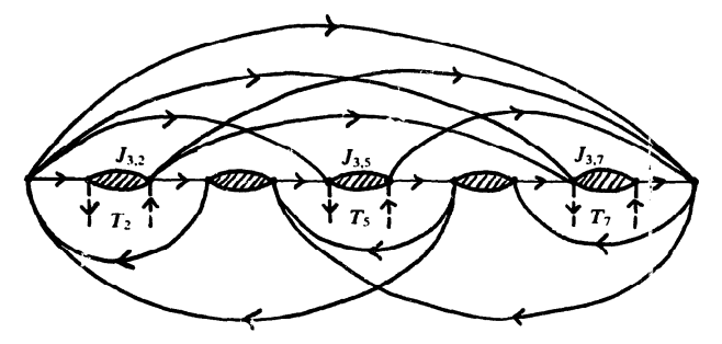
Now observe the interchanges. Each interchange has 5 junctions, 3 of which are connected to a corresponding track, which consists of the variable that is present in that particular clause, and 2 are internal junctions, which are of the same structure as a normal junction. A careful observation tells us that the whole of an interchange (all the five junctions) cannot be picked up by a route, in fact, all 3 of the external junctions can never be picked up in a route by the interchange, so at least one of the 3 junctions connected to tracks must be picked up by a track, this constraint being synonymous to the fact that we need at least one literal in the clause to be true, to make the whole clause true.

Now the total number of good routes (cycle covers) exactly corresponds to the total number of satisfying variable assignments for the boolean formula \(F\) of the SAT instance we had taken. Since #SAT is known to be #P-complete, the Permanent problem is now proved to be #P-Hard.

Let’s get on to finding the permanent of a 0-1 matrix now. It is a great thing to note that though the problem of finding a perfect matching in a bipartite graph \(\in\) P, yet counting the total number of perfect matchings \(\in\) #P-complete. This is one of those examples where it becomes clear that easy decision problems can have very hard counting versions of themselves. Rest of the post is about proving that 0-1 permanent is #P-complete.

To prove this, we will reduce the permanent problem to the 0-1 permanent problem. First, we need to make the weights of all the edges non-negative. Doing this is easy with modular arithmetic. We can compute \(permanent\ mod\ r\) for all \(r = \{2, 3, 5, 7, ... p\}\) where \(p \leq M^n n!\), as we do not need to consider primes greater than the largest value the expression of the permanent can take. Here \(M\) is the maximum value in the matrix, so a total of \(n!\) permutations of the entries with each of them being equal to the maximum value. That’s the maximum we will ever have.

Since the number of primes \(\leq M^n n!\) is \(\leq \log_2(M^n n!) \approx n \log_2M + n \log_2n\), the complexity is polynomial in terms of input size for this reduction. We can reconstruct the permanent using CRT.

So now we have a matrix where all the entries are non-negative. We have to reduce this to a form where all entries are either 0 or 1, to prove that the permanent problem is reducible to the 0-1 permanent problem. We can do so in two ways, by transforming the original graph to an equivalent graph.

• As mentioned in the original paper, Fig. 2 by forming self-loops proportional to the weight of the edge.
• First, convert all the edges to widgets such that all the edges in the resultant graph have weights which are powers of 2. Then all edges that are powers of 2 can be easily transformed to widgets where we only have 0-1 edges. All the while proving that the initial and final graphs are equivalent.

The first method is mentioned in the paper, so I will be explaining the second perspective here. Images are taken from Wikipedia. First, we transform the graph \(G\) into one where all edge weights are powers of 2, the graph \(G^{'}\). To do this, we take an edge with weight \(w\) and split it into a widget as shown in the image below. We use the fact that any number can be expressed as a sum of powers of 2.

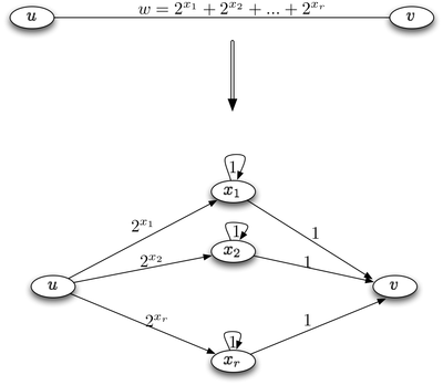
To prove the correspondence, take two cases for a cycle cover C of the graph \(G\):

• If edge u-v was not in C, then to cover all the edges in the transformed graph, we must use all the self-loops, so the total contribution = 1 in the product, and hence we have no change in the output. This is as good as not considering the edge u-v in the original graph
• If edge u-v was present in C, then in all the corresponding cycle covers in \(G^{'}\), there must be a path from u to v. We can see that there are total \(r\) such paths and they sum up to \(w\)

Hence graphs \(G\) and \(G^{'}\) are equivalent in terms of the permanent problem. Now we are left with a transformation such that all edges become binary, with weights 0 or 1. This is easy in the following way (Refer to the image below).

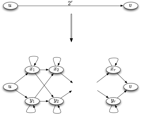
This is the transformation from \(G^{'}\) to \(G^{''}\). Again we have two cases to show the similarity. Let C be a cycle cover in \(G^{'}\), then:

• If edge u-v was not a part of C, the only way to form a cycle cover (taking all vertices) is to take all the self-loops
• If edge u-v was present in C, then in any cycle cover of \(G^{''}\) there must be a path from u to v. At each step from u to v, we have 2 choices, and such a choice has to be taken \(r\) times, so we have a total of \(2^r\) different possible paths from u to v, so it will contribute \(2^r\) overall, same as the weight of the u-v edge in \(G^{'}\)

Thus the problem of finding the permanent of a 0-1 matrix, and equivalently the problem of finding the number of perfect matchings in a bipartite graph \(\in\) #P-complete.

I have talked about more #P-complete problems and their proofs in this post.